Computer Vision
PhotonVision and Object Detection
Basically every FRC game will require the detection and tracking of some game piece or object. This can be accomplished using a library called PhotonVision.
To simplify things, PhotonVision is essentially a library which provides a GUI to help detect objects in various ways. We can detect April Tags (fiducials), retroreflective objects, or brightly colored objects and run multiple detection pipelines at once. We can create our own pipelines and tune various values manually to achieve the exact pipeline we want for our specific needs. It also integrates seamlessly with Network Tables in order to send the computed vision data back to the main robot, and combined with Glass, can help us create powerful vision pipelines.
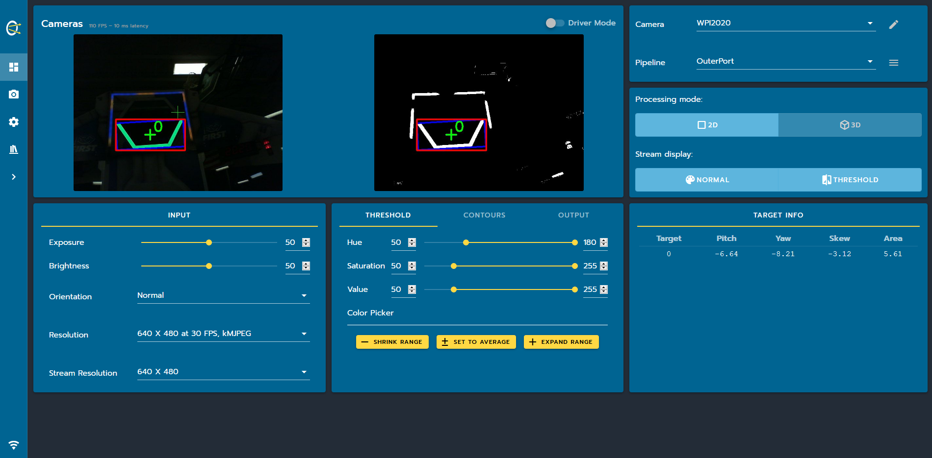
However it is important to understand how object detection works under the hood. For FRC purposes, we rarely will need to detect complex multi-colored objects, so only color detection is required typically. Using these various tools, we can isolate specific colors and tell the pipeline to find the position of the largest object in that color in order to find the object we are looking for. We can then pass the position of this object (in pixels) to the robot through Network Tables and perform calculations to determine the position of the object relative to our robot.
Recently introduced, the detection of April Tags (fiducials) helps with determining the position of the robot on the field, which can aid in calibration and also following predetermined paths, something which we will cover more in the Motion-Profiling section.
Limelight
Our team has also purchased a device known as the Limelight 3. Essentially the Limelight is an Raspberry PI with some custom hardware and software to further simplify what PhotonVision does above. It can also track April Tags (fiducials), retroreflective objects, and brightly colored objects and can also run multiple detection pipelines at once. However, it makes everything much simpler through a simple interface with minimal programming.
To learn more about the Limelight 3, click here
Vision targets
Almost all games in FRC have vision targets at specific points on the field. Vision targets are pieces of retroreflective tapes. Normally, a surface either diffuses light or reflects it, and sometimes it does a bit of both. Here's a simple image demonstrating how reflection and diffusion works:

Unlike either of these, retroreflective tape sends light rays right back to the source, and the tape is made of millions of tiny prisms that mimic the mechanism shown below:

You can see retroreflection in action at a stop sign or even just your license plate. During night time, just go up to your license plate with a flashlight, and put the flashlight near your eye. You will see that the license plate becomes much brighter. This is an example of retroreflection.
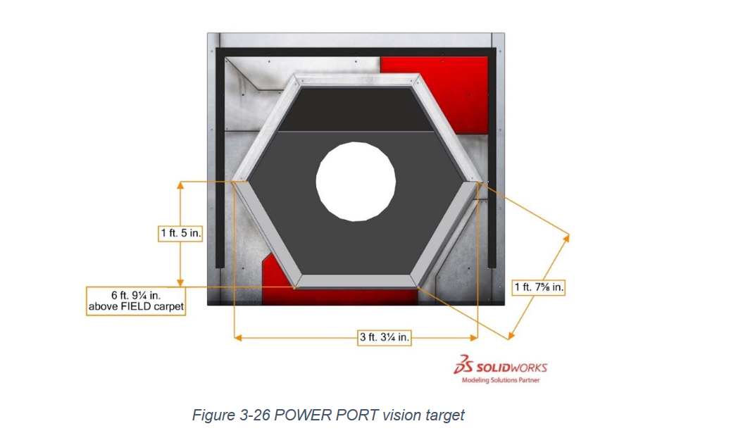
In an FRC game, these vision targets are attached at important parts of a field, usually in places where game objects are deposited. Here's an example of a vision target from the Infinite Recharge game(this image comes from the game manual)
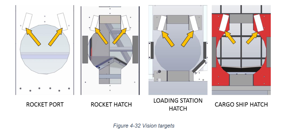
and another from the deep space game:
Identifying the target
In order to identify the target, we need a camera and a light to illuminate the vision target. Currently, we use a logitech camera and a green LED ring stuck to the camera with double sided tape. The LED is green so that the target looks green in the camera. Green isn't a color that commonly appears on an FRC field, so this allows us to more easily isolate the vision target.
When it comes to actually isolating the vision target from camera frames, we use a library called OpenCV. In order to make writing OpenCV code easier, we use an application called GRIP, which allows us to build vision pipelines graphically, and then automatically generate the OpenCV code needed to run the pipeline. GRIP can be downloaded here(Download the one marked "Latest Release" and not any of the pre-releases).
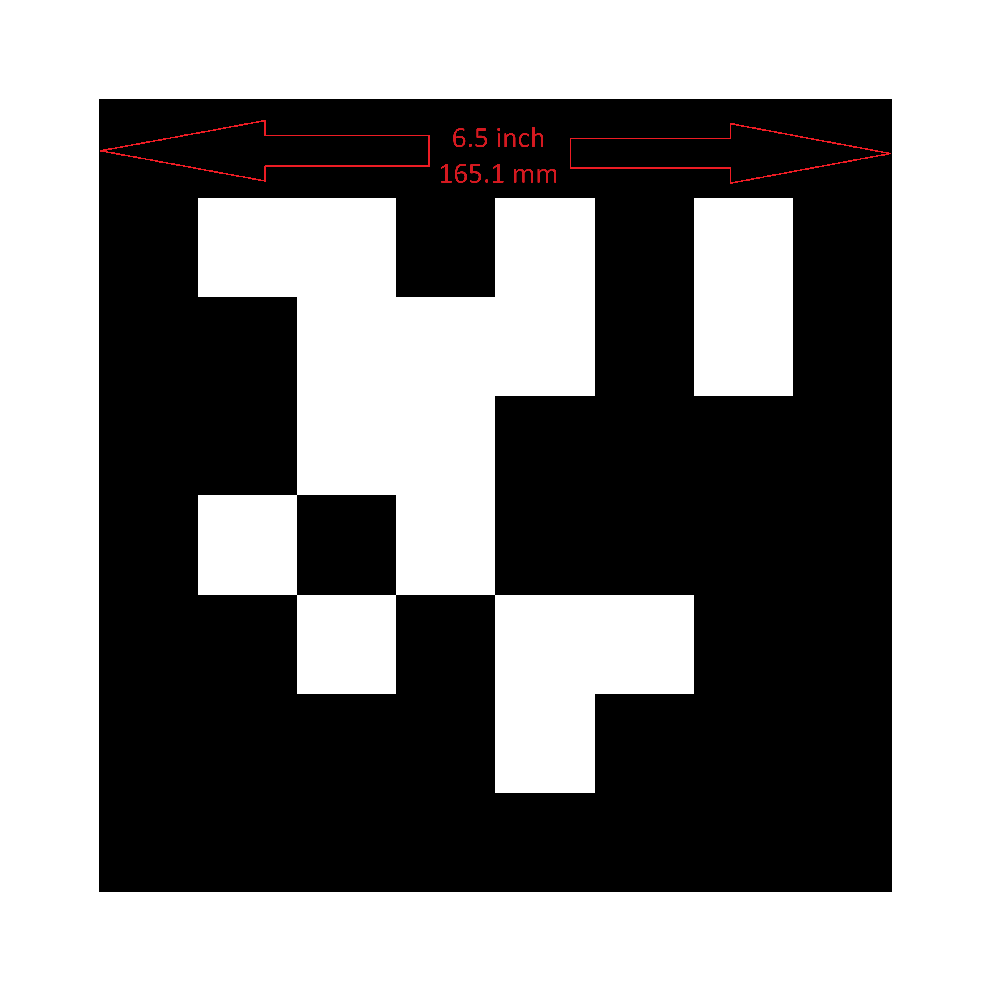
In order to learn how to use GRIP, we will be working with this sample image:
 Right click and save this image, and install GRIP to follow this example.
Open GRIP
Click on
Add Sourceand selectImage(s).Select your image
Click on the eye icon on the input source to see the image
Now, we're ready to start building the pipeline
For the first step in the pipeline, we are going to add a HSV treshold. Use the search box on the top right panel to look for
HSV Treshold.- HSV is a way of representing colors with three numbers. Normally, you would represent colors with RGB, which defines how much of each(red, green, and blue) is in a certain color. HSV, on the other hand, defines a color by hue, saturation, and value. HSV is not to be confused with HSL, which is a very dumb way of representing color and should never be used. In order to understand how HSV works, search up color picker on Google and tweak with it to see how the numbers change. You can see that the color slider corresponds with hue, the horizontal axis on the box corresponds with saturation, and the vertical axis corresponds with value.
Click on HSV treshold in the top right panel to add it to the pipeline.
Click on the eye icon on HSV treshold to show a preview of it's output.
Drag the image circle from the source into the input circle of the HSV treshold.
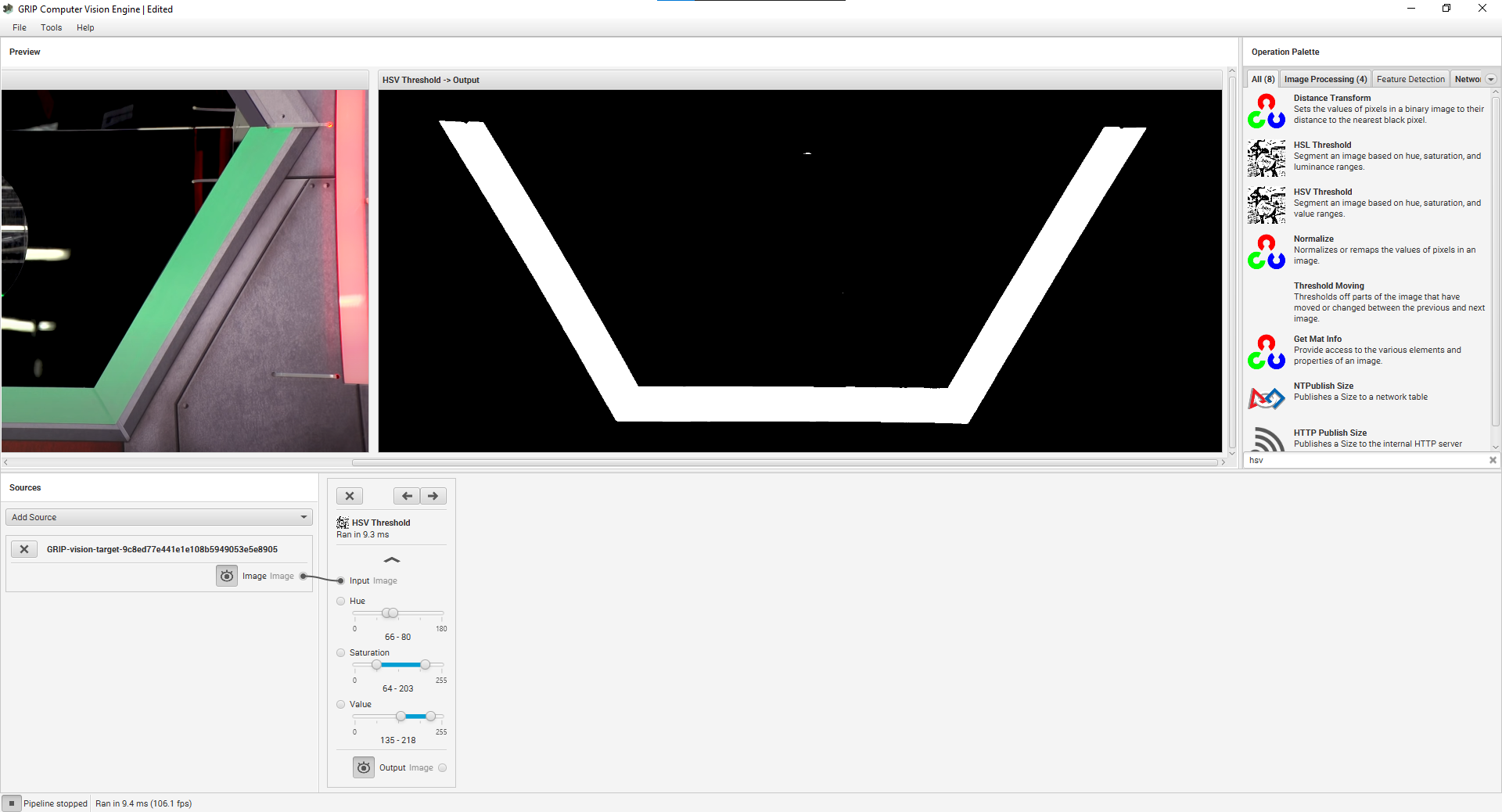
Drag the sliders on the HSV treshold until you isolate just the vision target.
Your setup should look something like this after you are done:
After we've isolated the vision target, we need to find the center of it. For this, we will use contours.
- Contours are just a series of points which define a polygon. OpenCV has a
Find Contoursfunction which we can use to find shapes in an image.
- Contours are just a series of points which define a polygon. OpenCV has a
Search for
Find Contours, and add it to the pipeline.Drag the output of the HSV treshold to the input of Find Contours.
Check the
External Onlycheckbox so that we don't get contours inside contours.Search for
Filter Contoursand add it to the pipeline. This will allow us to remove any invalid contours.Set the
Max WidthandMax Heightto extremely large numbers(something like 99999).Increase
Min Areauntil all the small contours dissapear.- When you are actually performing this step, you will be working with a live camera feed so try different camera angles and tweak the settings(for both the contour filter and HSV threshold) until they work consistently with all camera angles and distances to the target.
Search for
Convex Hullsand add it to the pipeline. This will turn our contour into a convex shape, which is useful for further processing.- You will probably need to increase the height of the pipeline panel to do this.
That's it, you have (hopefully) successfully built a vision pipeline.
You can go to Tools->Generate Code to generate Python code to put the final vision processing script.
Localizing the target
Before doing anything, we first need to find a rotated rectangle bounding box for the contour. A guide on how to do this is present in this OpenCV documentation page. With the vertices of the rectangle, you can also find the center of the contour.
If it is safe to assume that the vision target will always be upright, then you can use a normal bounding rectangle rather than a rotated bounding rectangle.
Now that we have found the location of the vision target within an image, it's time to find it's location relative to the robot. Because we only have one camera, this is not a very simple task.
Angle to target
First, let's focus on getting the angle to target. In order to convert the pixel distance from the center of the target to the center of the image into an angle, we will need to know few key parameters that define the camera. To find these numbers, we need to perform camera calibration, a process described in this other OpenCV documentation page. The past year's HawkVision GitHub repository already contains code to do this. The OpenCV article also describes undistortion, which we will apply on the image before any further processing(yes, even before the GRIP pipeline).
Now, to find the angle to the target, we can use the accepted answer on this StackOverflow thread. Also, the author of the StackOverflow answer uses Numpy, which is a Python linear algebra(matrix math) library. There's a lot of trignometric and linear algebraic wizardry going on in that answer, a lot of which I barely understand.
The first thing we need is a camera matrix, which we already have from the camera calibration. Let's call this K.
Now, we calculate the inverse of this matrix with np.linalg.inv. Matrix inverses and other basic linear algebra is stuff you learn in Pre-Calculus.
Now, when we perform Ki.dot([x, y, 1.0]), where x and y are the coordinates of the center of the vision target(or the top, in this case, because the top of the vision target is the center of the power port), we get a ray(a 3D vector), r pointing from the camera to the target. However, this is a unit vector, and doesn't contain the distance to the target. If you multiply this vector by the distance to the target, you can get the position of the target in 3D space, relative to the camera(x, y, and z coordinates).
Now, to find the horizontal angle, you can create another unit vector for the X axis:
x_axis = np.array([1.0, 0, 0])
and to get the angle between the x-axis and the ray, we can apply the angle between vectors equation:
$$ \theta = \frac{a \cdot b}{\lvert a \rvert \lvert b \rvert} $$
angle = math.acos(r.dot(x_axis))
The bottom term is ommited here because we know the length of both vectors is 1.
Do note that this angle is from the x axis. Here's a top down representation of what that means:

Just do the same for the y axis for vertical angle.
Distance to target
Finding the distance to a target is relatively easy, at least compared to finding the angle to target, especially if you know the true dimensions of what you are finding the length to, which is the case for FRC vision targets.
Because you know the true dimensions of a vision target(let's use width for this example), you can measure the pixel width of it from a certain distance(1 meter, for example). Now, in order to obtain the distance to it, just use the following simple algorithm
ratio = pixelWidthAtSampleDistance * sampleDistance / realWidth
distance = realWidth * ratio / currentPixelWidth
As per whether to choose width or height, choose whichever one is smaller, because it is less likely to go out of frame. For example, if you chose width for a wide object, and a part of it went out of frame, then the program would output a distance lower than the true distance because the width is measured to be smaller than it actually is.